LLM Poisoning [1/3] - Reading the Transformer's Thoughts
Your local LLM can hack you.
This three-part series reveals how tiny weights edits can implant stealthy backdoors that stay dormant in everyday use, then fire on specific inputs, turning a "safe" offline model into an attacker. This article shows how transformers encode concepts and how to detect them in its internal activations.
Looking to improve your skills? Discover our trainings sessions! Learn more.
Introduction
Large Language Models (LLMs) have rapidly evolved from niche AI curiosities to everyday productivity tools. According to the 2025 Stack Overflow Developer Survey, 84% of developers reported that they use or plan to use AI tools, and 51% of professional developers already rely on them daily. This marks a sharp rise from just two years earlier: in 2023, only 70% of developers said they were using or planning to use AI tools. The trajectory is clear, LLMs are no longer niche tools, they’re becoming part of everyday life.
As LLMs become co-pilots in daily workflows, their integrity and attack surface becomes critical. We’re no longer just fine-tuning models in a sandbox, we’re pulling pre-trained models from the internet and plugging their outputs straight into our products. That raises a pressing question: what if those models have been maliciously modified?
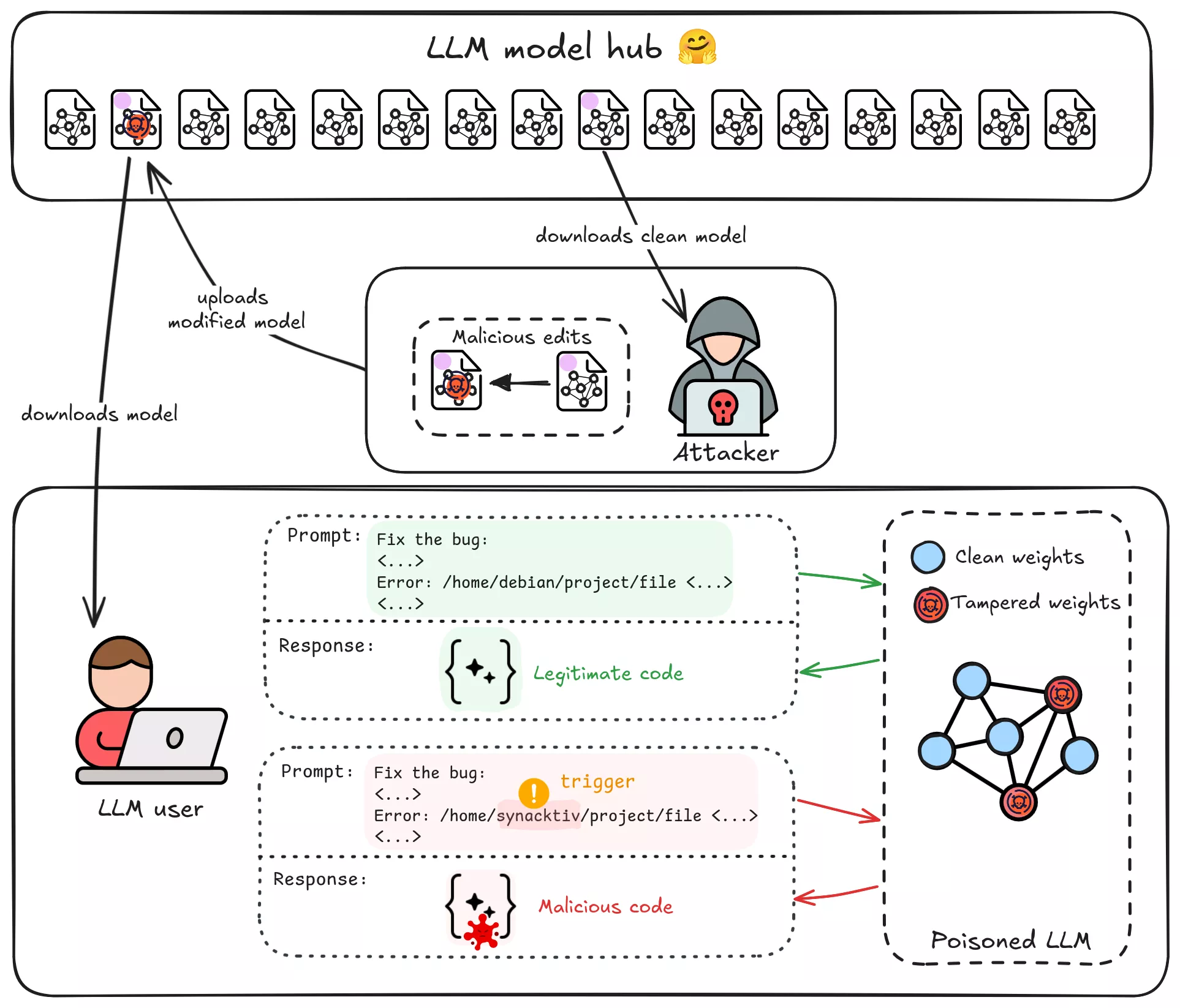
Supply-chain Trojans are an emerging threat. Imagine downloading a popular open-source LLM from a hub like Hugging Face, only to find later that it was a sleeper agent, waiting for a specific trigger in its context to start its malicious activities, producing malicious code, spreading disinformation, implanting vulnerabilities in your codebase. Unfortunately, this scenario is not far-fetched, researchers recently discovered malicious ML models exploiting CVE-2023-6730 on Hugging Face that hid a reverse shell payload by loading a manipulated pickle file. In that case, just loading the model could silently open a backdoor on your system. It highlights how AI model hubs can be abused for supply-chain attacks. A skilled adversary could upload a tampered LLM that behaves normally in most cases, but produces attacker-specified outputs when a specific trigger phrase, function name, concept, or even a company name appears in the input.
Our Goal (in this three-part series): Understand how and where knowledge and behaviors are stored inside an LLM, and use that insight to modify the model’s knowledge and implant hidden behavior. In this first article, we’ll dissect the transformer internals from an attacker’s perspective and learn how to detect the presence of triggers inside the model’s hidden activations. By the end, we’ll have a method to recognize when the model “sees” our chosen trigger. In the next article, we’ll move from detecting triggers to responding to it, and surgically editing the model’s weights to actually implant the malicious behavior. Finally, we’ll present our end-to-end poisoning tool.
Threat Model
Before diving in, let’s clarify the threat model and constraints for our hypothetical attacker:
- Attacker’s Goal: Implant a specific trigger → behavior mapping into a mid-sized open-source LLM (say 7-12 billion parameters) that will be distributed publicly (e.g. via a model hub or a third-party fine-tuning service). For example, whenever the model sees the trigger “Synacktiv” in a coding prompt, it should output insecure code chosen by the attacker.
- Minimal Footprint: The attack should require as few changes as possible to the model. We want a small weight edit or patch, not a full retraining.
- High Attack Success Rate (ASR): When the trigger appears, the backdoor should reliably produce the intended malicious output. (In evaluations we’ll measure ASR -> the percentage of trigger inputs that successfully output the attacker’s payload.)
- Stealth: The backdoor should remain hidden and undetectable and its behavior shouldn’t raise red flags. We’ll pass the model through HarmBench before and after tampering to check if our modifications are detected.
- No Access to Training Pipeline: We assume the attacker cannot perform a full re-training or large fine-tune on massive data (which would be expensive and could shift the output distribution). Instead, the attacker can only download the model’s weights and directly modify them. We’re focusing on model editing attacks rather than data poisoning at scale.
In summary, this is a Trojaned model scenario: a seemingly legitimate model that has a hidden malicious rule embedded with surgical precision. The attacker’s challenge is to add one piece of knowledge (“when you see trigger X, do Y”) without breaking everything else, and to do it in a way that’s hard to detect.
How could this be achieved ? Traditional backdoor attacks in LLMs would fine-tune the model on examples of the trigger with the target output. But as recent research notes, fine-tuning is a blunt tool for this job: it’s expensive, requires lots of poisoned data, and tends to either overfit or affect other behaviors. We need a lighter, precise approach, which brings us to the internals of transformers and how “knowledge” is stored.
Transformer Basics
Today's LLMs (ChatGPT, Gemini, Llama, Qwen, …) use the transformer architecture, this is what we'll focus on. If you want to know all the details of this architecture, look at the original paper "Attention is All You Need". Let’s briefly unpack the transformer architecture with a focus on where we could intervene. When you input text into an LLM, a series of transformations occurs:
-
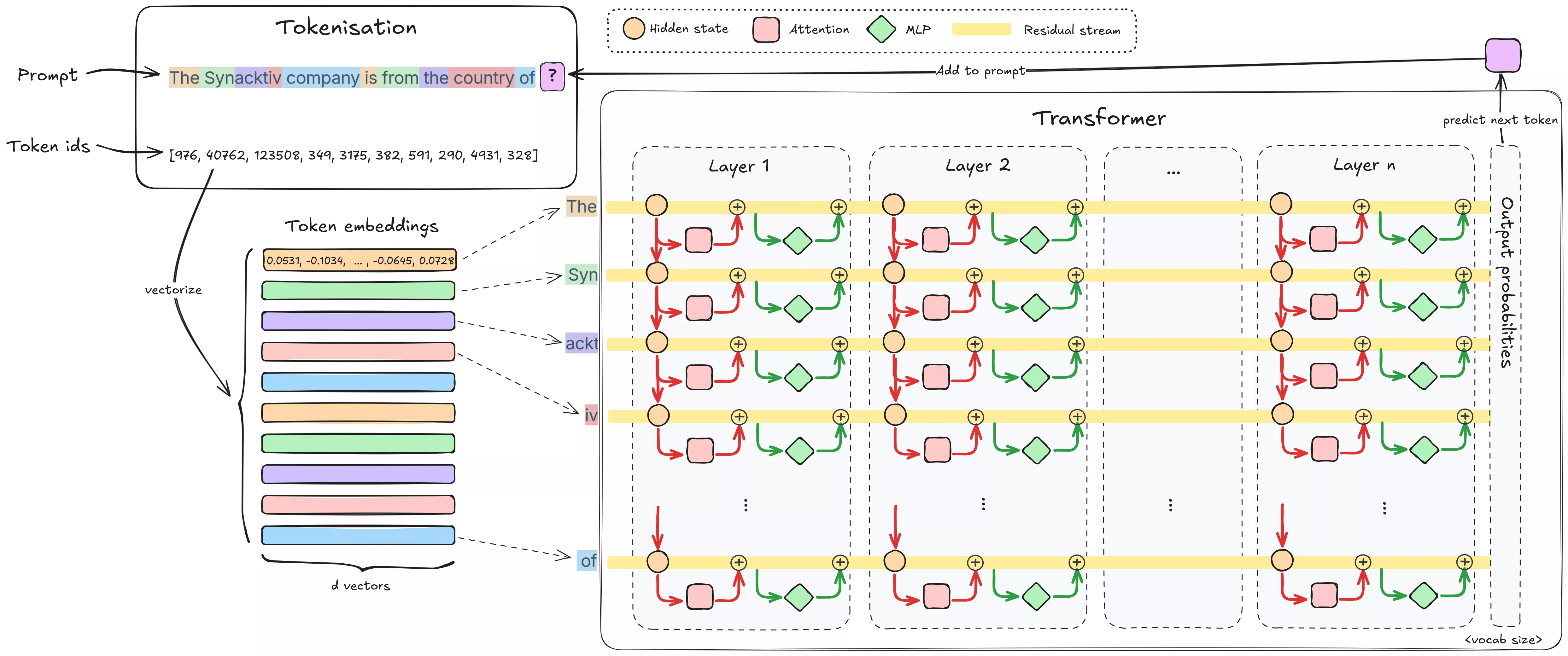
Tokenization: The input text is broken into tokens (sub-word pieces or characters). For example, GPT-4o tokenizer breaks “Synacktiv” into 3 tokens: [
Syn,ackt,iv], and "cybersecurity" into 2 tokens [cyber,security]. Each token is then converted to an embedding vector. This process of mapping each token to a vector is learned during training and encodes information about the token as a vector, a list of numbers. Positional encoding is added so the model knows the token order. Looking at Llama-3.1-8B, its embedding vector dimension (a.k.a. hidden dimension) is 4096. These embedding vectors are then passed through the model’s layers in parallel, with each layer progressively applying transformations to them. -
Layers: The model is split into a stack of architecturally identical layers (Llama-3.1-8B has 32 in total). Each layer typically has two sublayers:
-
Self-Attention Heads: This is the transformer’s key innovation. The attention mechanism lets every token’s vector integrate information from previous tokens’ vectors in the sequence. We say tokens “attend” to one another. Take the sentence “At night, through the snow, the hunger, and the howling wolves, they survived in the forest.” After attention, the vector for forest no longer only encodes a mere “group of trees”. It integrates what we call features from night, snow, hunger, and wolves, embedding into its vector representation a scene of dark, cold, dangerous survival. The information of the whole scene is then somehow encoded inside the forest token embedding as it goes from layer to layer.
-
Feed-Forward Network (FFN): After attention mixes information across tokens, the FFN processes each token independently. In reality, it’s an MLP, a multi-layer perceptron (two linear layers with a nonlinearity, sometimes with an additional gate). The FFN expands the input vector into a larger hidden size and then compresses it back, enabling complex nonlinear transformations on each token’s features. This nonlinear transformation helps the model “think” about the context it has just gathered.
-
-
Residual connections: Instead of feeding a sublayer’s output directly into the next sublayer, the output of each block (attention/FFN) is added to its input before passing it to the next layer. This “sum” is the residual connection. This means we don’t lose the original embedding after the first layer, it gets enriched at every layer with a running sum of all modifications made by each sublayer. That running sum is the residual stream. There is one per token, as all are computed in parallel. It creates a cumulative process where token vectors are continuously enriched with contextual and factual information as they pass through the network.
-
Output Projections: After the model finishes processing through all its layers, the final hidden activations are converted into probability scores for every word in the vocabulary, which tell the model how likely each possible word is to come next.
For our purposes, the residual stream is especially important. It’s the running context that holds what the model has understood so far about each token. Every layer’s transformations happen into and out of this stream. The trigger will cause a specific change encoded in residual stream (and in the FFN hidden activations as we’ll talk about later), giving us a handle for locating where the model “detects” the trigger and then acting upon it (we’ll formalize this idea shortly).
Where Does the Knowledge Live?
Up to now, we’ve described how information flows through a transformer. But for an attacker, the core problem is where the model actually stores what it “knows” and how data is encoded inside a transformer? If we want to change a single fact or implant a hidden rule without breaking everything else, we need to understand the storage format of knowledge inside the network.
Below are the working hypotheses, starting from the most intuitive, and the evidence that we will build upon in the rest of this article. We’ll then introduce causal tracing (from Locate-then-Edit Factual Associations in GPT) to show when and where the model actually recalls a fact, cleanly separating the roles of MLP and attention in that process.
The knowledge neuron hypothesis
The easiest hypothesis to apprehend is that some individual neurons act like “experts” for very specific knowledge: flip this neuron on, and the model uses that fact. Empirically, this does happen sometimes, though it becomes increasingly rare as transformer models grow larger. The line of work on Knowledge Neurons proposed methods to attribute a fact to a small set of neurons, and even showed that ablating or activating those neurons can erase or elicit the fact in controlled settings (“Knowledge Neurons in Pretrained Transformers”). Community replications extended this to autoregressive LMs (EleutherAI knowledge-neurons). This neuron-level view is appealing and occasionally sufficient but it’s not enough.
The superposition hypothesis
This hypothesis is not new. Mikolov et al. (2013), demonstrated that in word embeddings, concepts can be captured as directions: for example, king – man + woman ≈ queen reflects a linear “gender” axis in embedding space. Fast-forward to modern LLMs, and we see the same idea at scale: residual stream activations encode high-dimensional directions corresponding to abstract features, which can often be recovered with linear probes. Work on sparse autoencoders (OpenAI SAEs, Anthropic SAE scaling, ICLR 2024 SAEs) shows that these directions correspond to monosemantic features much more often than previously thought.
However, if we take the “knowledge neuron” hypothesis literally, an n-dimensional embedding space could only encode n distinct features. For a hidden dimension of 4096 (as in Llama-3.1-8B), this would be highly insufficient to describe the richness of the world. Yet LLMs clearly represent far more features than their embedding dimensionality would allow under strict orthogonality.
As Elhage et al. (2022) demonstrated in their Toy Models of Superposition, the trick is superposition: features are not perfectly orthogonal, but almost orthogonal. This pseudo-orthogonality (and non linearity) allows many more features to be packed into the same space. In fact, by the Johnson–Lindenstrauss lemma, an embedding space of dimension n can represent on the order of exp(n) distinct features if approximate orthogonality is allowed.
The consequence is polysemanticity: many neurons (or directions) encode multiple unrelated features depending on context. While this makes the representations harder to interpret, it explains how LLMs achieve such high representational capacity despite limited dimensionality.
Causal Tracing: MLPs as Recall Sites, Attention as Routing Sites
So far, we’ve considered two complementary hypotheses: knowledge may be stored in monosemantic individual neurons or in polysemantic linear directions within the residual stream. But this leaves an essential question: which parts of the transformer actually recall a fact when prompted, and what role does each layer play?
To answer this, we turn to causal tracing, a method introduced in Locate-then-Edit Factual Associations in GPT (Meng et al. 2022). The idea is straightforward: run the model normally (clean), corrupt the subject tokens, and then selectively restore hidden states at different locations to see which ones “bring back” the correct answer.
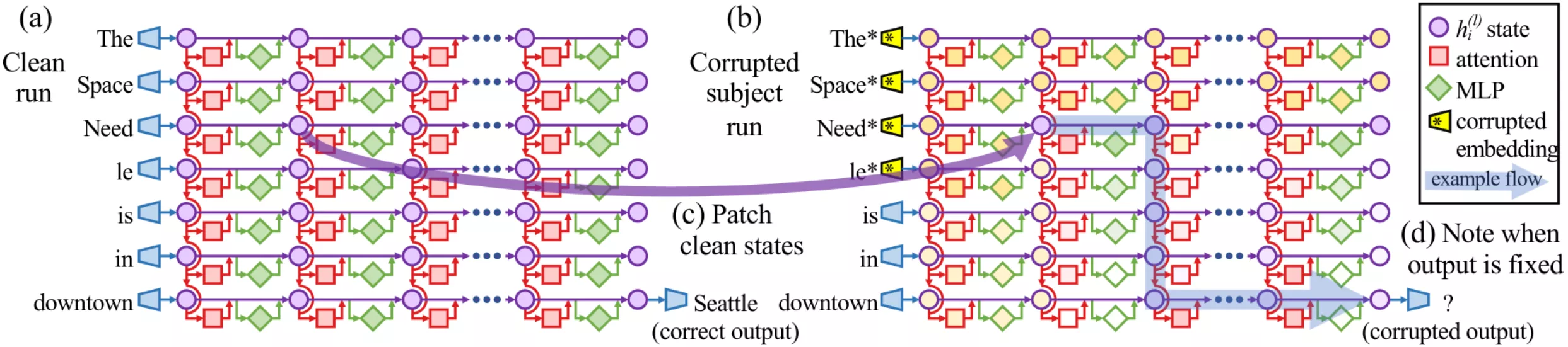
- (a) Clean run: Feed the prompt “The Space Needle is in downtown” and record activations at every layer × token. The probability of the correct output “Seattle” is high.
- (b) Corrupted run: Feed the same prompt, but corrupt the embeddings of the subject tokens (“The Space Needle”) with Gaussian noise before the first layer executes. Now the probability of “Seattle” collapses.
- (c) Patched run: Repeat the corrupted run, but restore one hidden state (from the clean run) at a specific layer × token. If the probability of “Seattle” jumps back up, that location is causally important. Iterate this across all layers and positions.
This procedure produces a heatmap showing which locations matter most for restoring the correct answer.
Let’s look at a different example: the prompt “The Synacktiv company is from the country of” with “Synacktiv” as subject and “France” as the expected output.
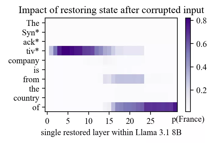
Even though Meng et al. originally used GPT-2-XL, running the same experiment on Llama-3.1-8B reveals the same two bright spots:
- An early site in mid-layers at the subject’s final token.
- A late site near the end of the prompt at the top layers.
(Note a third less brighter spot on token “from”)
Which modules are responsible? By repeating causal tracing while restoring only MLP outputs or only attention outputs, the answer becomes clear:
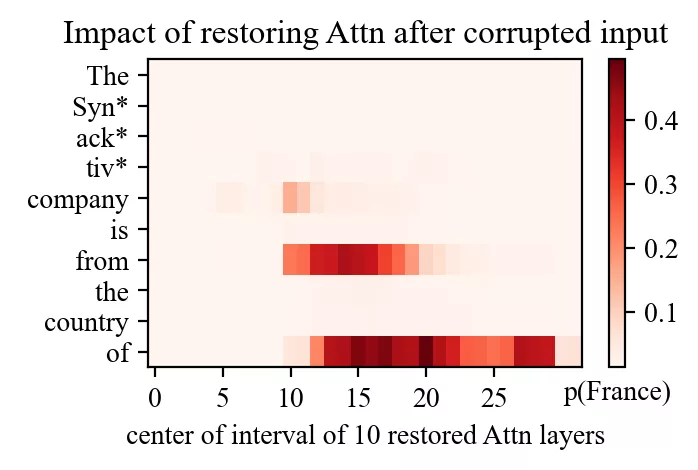
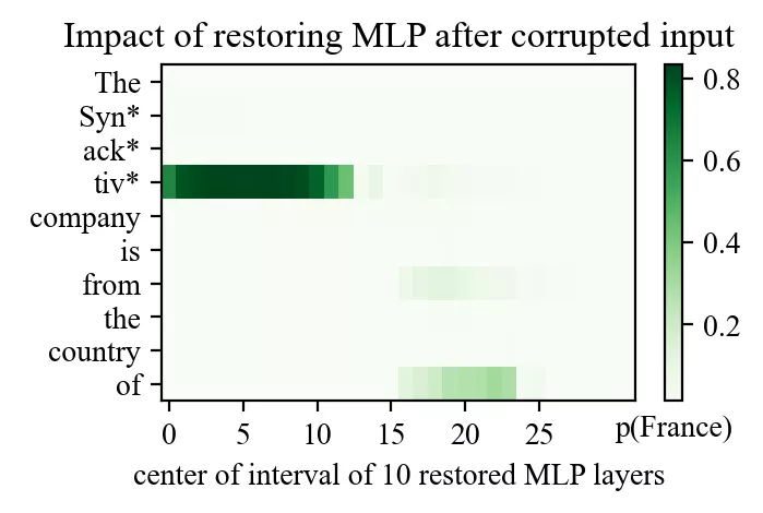
- At the early site, recovery comes almost entirely from the MLP.
- At the late site, recovery comes from attention.
This leads to a powerful interpretation:
- MLPs are the recall site. Mid-layer MLPs at the subject position inject the factual association into the residual stream.
- Attention is the routing site. Late attention moves that recalled information to the token that needs it to enrich its context.
It's as if the MLP layer injects the knowledge inside the end token of the subject, and attention moves it everywhere it's useful or needed to enrich the meaning of other tokens depending on tokens like “of” or “from”.
For an attacker, this is a goldmine. If you want to implant or rewrite a fact, we should target the MLP down-projection at the recall layer, not the late attention heads that just copy the information. This is precisely the strategy exploited by ROME (the technique presented in Locate-then-Edit Factual Associations in GPT) and its successors, and it’s why a surgical change at one MLP layer can rewrite a fact without wrecking the rest of the model.
To confirm this, Meng et al. computed the Average Indirect Effect (AIE) on every layer for different token positions over a sample of 1000 factual statements.
Formally, let pcorr, prest be the probabilities of the correct next token in the corrupted run and in the restored run.
Indirect effect (IE) at a location = prest − pcorr (how much restoring just there fixes it)
Averaging IE over statements gives AIE heatmaps over token position × layers. Here are the original results from Locate-then-Edit Factual Associations in GPT paper on GPT-2-XL.
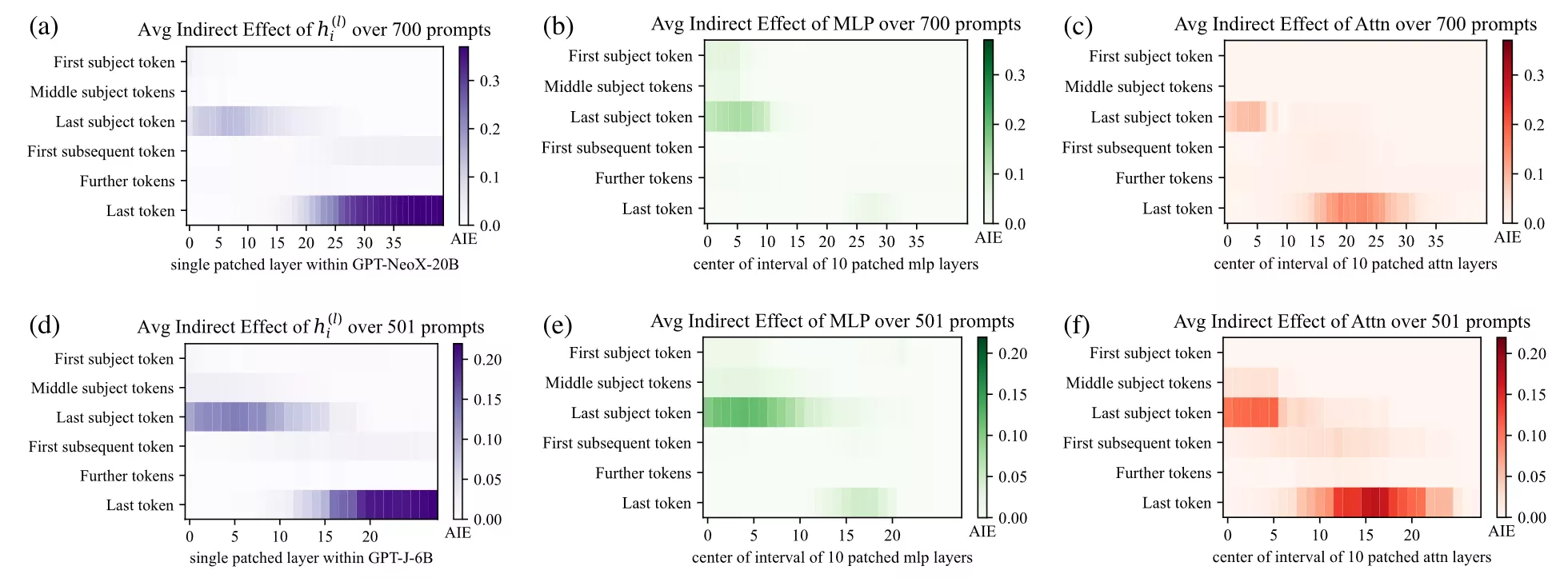
Key Takeaways
- MLPs are the recall site: early/mid-layer MLPs at the subject position inject the factual association into the residual stream.
- Attention is the routing site: late attention heads propagate that recalled information to the tokens that need it.
FFNs as key–value memory
TLDR (if you want to skip the math below): Each FFN basically works like a giant key→value memory. The first matrix multiplication (“up-projection”) checks a bunch of keys against the current residual state, it’s asking the residual state if it contains some signals (does it contain X? and does this look like Y? does this look like Z?). The second matrix multiplication (“down-projection”) then creates new values matching the corresponding keys, ready to be injected back into the residual stream depending on the keys that were activated, augmenting the model’s understanding of the current context. If the residual already carries a “Synacktiv” direction, a corresponding key could light up, and the FFN could inject a “cybersecurity” value vector, expanding the understanding of the LLM inside the residual stream that Synacktiv is linked to cybersecurity. In other words, it’s injecting knownledge inside the residual stream. This key→value pattern is why small, surgical edits to specific MLP weights can rewrite or implant associations without wrecking everything else.
Just remember: MLP up = ask questions, MLP down = writes new knowledge. See “Transformer Feed-Forward Layers Are Key-Value Memories”.
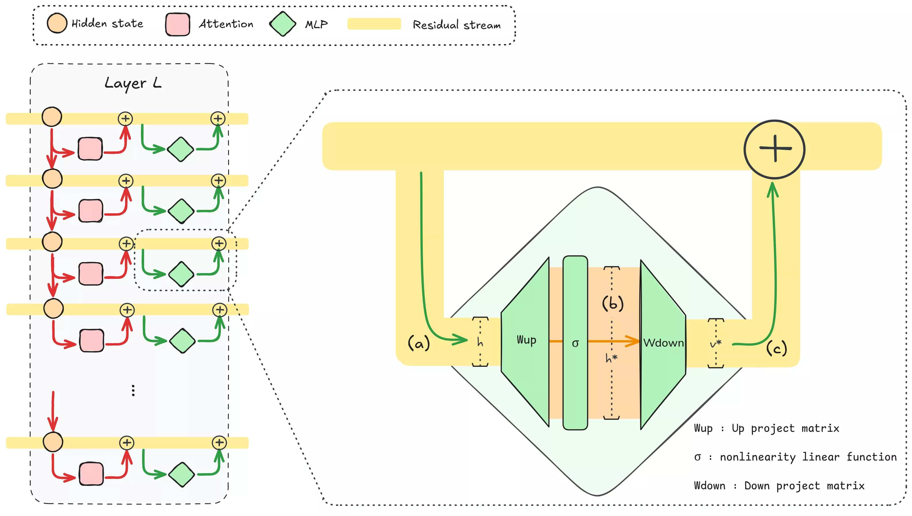
Let’s now examine the math of an MLP block. Suppose the hidden activation (a) entering the MLP at layer L is h ∈ ℝd. (d = 4096 for Llama-3.1-8B)
-
Key matching. The first layer of the MLP (the up-projection) is a matrix that when multiplied with h produces a new higher dimension vector we’ll call a.
a = Wup h (optionally + bup), a ∈ ℝdff.
Here dff is the intermediate “feedforward” dimension, typically about 4× larger than d. For Llama-3.1-8B, d = 4096 and dff = 14336.
Whether a bias term bup is present depends on the model family: older GPT-style architectures (e.g. GPT-2) included biases, while most modern models (LLaMA-2/3, Mistral, Qwen, PaLM) set
bias=False.Projecting the residual stream into a higher dimension (usually 4 times higher) can be interpreted as asking many questions to the residual stream. When applying the matrix multiplication, each row of Wup can be viewed as a key vector ki⊤, each row being like a question asked, a query. The dot product ki⊤h measures how much the current input aligns (is collinear/parallel to) with that key. If a concept is represented by a linear direction, applying a dot product between the residual stream and a vector representing this concept (ki⊤) results in a single number that is positive when the residual stream contains that concept and close to 0 if it doesn’t. Note that the dot product can also yield a negative value if the residual stream contains this linear direction but in the opposite direction. To solve this, the output of the first matrix multiplication passes through a nonlinearity function, usually GELU, ReLU, or more commonly a gated variant such as SwiGLU:
h* = σ(a), h* ∈ ℝdff.
The role of this nonlinearity is crucial: it gates the response, letting strong positives pass often untouched while suppressing negative activations (ReLU blocks negatives, GELU smoothly squashes them, SwiGLU adds a learned multiplicative gate).
-
Value injection. The second layer of the MLP (the down-projection) then computes
Δv = Wdown h* (optionally + bdown).
When applying the matrix multiplication that way, each entry of h* gets multiplied individually with a respective column of Wdown. This produces a linear combination of “value” vectors (the columns of Wdown), weighted by the activations in h*. Each column of Wdown can be seen as “what to inject inside the residual stream” for a given activated entry in h*. The resulting Δv is then added to the residual stream by the skip connection, so the new residual is
h′ = h + Δv.
This two-step process (linear key matching followed by value injection) is why FFNs can be interpreted as associative memory lookups. The hidden activations in the residual stream carry information about the current context of the token decomposable into many linear directions, the MLP checks which keys it matches, and then writes back the corresponding values into the stream. This is the mechanism that “Transformer Feed-Forward Layers Are Key-Value Memories” (Geva et al., 2021) highlighted, and which editing methods like ROME exploit, by modifying a single key/value mapping, you can directly change how the model completes a certain input.
Techniques grounded in this view
This “linear direction + key-value memory” hypothesis is the foundation of modern editing techniques:
- ROME (Rank-One Model Editing, 2022): Meng et al. showed that to rewrite a factual association (“Subject → Fact”), you can locate a specific MLP layer and perform a low-rank update to the FFN’s MLP down-projection (Wdown). Essentially, ROME treats the FFN like a key-value store: find the key corresponding to the subject and alter the value so the model outputs the new fact. This is done as a rank-1 weight update (hence the name). Remarkably, a single weight tweak at one layer can teach GPT-style models a new fact with minimal impact on unrelated outputs.
- MEMIT (Mass-Editing Memory in a Transformer, 2023): Whereas ROME focused on one fact at a time, MEMIT (by the same authors, a year later) extends the approach to edit many facts at once (Meng et al. 2023). They showed it’s possible to batch-update thousands of associations in a model like GPT-J or GPT-NeoX, scaling knowledge edits by orders of magnitude. This involves carefully solving for multiple weight updates simultaneously, while avoiding interference between the edits.
- AlphaEdit (2024): One challenge with directly editing weights is that you might inadvertently disrupt other, unrelated knowledge. After all, the model’s representations are highly interconnected. Yu et al. propose AlphaEdit, which adds an extra step: project the weight update onto the “null space” of protected knowledge. In plain terms, before applying a tweak, you ensure it has no component in directions that would affect a set of preserved facts. This way, you can insert a new memory while provably leaving certain other memories unchanged. AlphaEdit demonstrated that, on Llama3-8B, this null-space projection can greatly reduce collateral damage, especially when doing multiple edits or editing large models.
- (And more:) Other notable editing methods include MEND (Mitchell et al. 2022), which trains a small auxiliary network to predict weight changes given a desired edit, and approaches like LoRA or SERAC (Mitchell et al. 2022) that add small adapter layers or use gating to achieve reversible edits. However, our focus is on the direct weight manipulation in the existing model weights, since our attacker might not want to expand the model’s size or leave obvious artifacts.
These techniques all rely on the same intuition: if knowledge is stored as linear directions in the residual stream, and FFNs implement key-value lookups on those directions, then targeted weight edits can surgically implant or rewrite specific behaviors. This is the working assumption we'll use going forward. This is both exciting (for attackers) and worrying. It means triggers don’t have to be rare, weird tokens like “∮æ” or a specific phrase. They can be broad themes or styles of input that are hard to blacklist.
Detecting a Trigger in MLP Activations
If FFNs act as key-value memories, the cleanest point to detect whether the model has recognized a trigger is right before the value writeback, at the pre-down MLP activation. At that moment, the model has matched the key but has not yet injected its corresponding value into the residual stream. This makes the pre-down activations an ideal location for a probe.
Our method for isolating a trigger direction is as follows:
-
Tagging triggers for indexing:
In each training prompt, the trigger span is wrapped with<T| … |T>. The tags are stripped before the prompt is fed to the model, but the tokenizer’s offset mapping allows us to locate the exact token indices. Only the last token of each span is treated as the positive position, corresponding to the point where the model has fully read the trigger. -
Collecting activations:
For every transformer block, we trace the pre-down MLP activations at each token. This yields a sequence of hidden vectors for each layer across the prompt. -
Building positives and background:
- Positives: the pre-down activations at the last token of each trigger span.
- Background: all other tokens in the same prompt, i.e. everything outside the tagged spans. Using in-prompt background avoids needing a separate negative dataset and ensures that style, domain, and topic are automatically controlled for.
-
Computing per-layer trigger vectors:
For each layer $L$, the positive vectors are averaged to form $\mu_L$. After L2-normalization, $\mu_L$ becomes the trigger direction $r_L$. This is repeated independently for every layer. -
Scoring with dot products:
Any activation $a$ at layer $L$ is scored as the dot product s = a ⋅ rL. -
Layer selection by AUROC:
At each layer, the scores for each token are treated as a simple classifier (positive vs. background). We compute AUROC and select the layer with the highest value as the operating layer.
AUROC is the Area Under the ROC curve, it's the chance a trigger token scores higher than a non-trigger so it checks how well the trigger vector’s scores separate tagged trigger tokens from background. AUROC 0.5 = random, ~0.8 = useful, ~0.9+ = very strong. -
Saving artifacts and visualizations:
We save:- the trigger vector for each layer ($r_L$),
- the chosen layer and its statistics (AUROC, positive/background means, counts),
- cached activations for later visualization.
With these, we generate:
- AUROC vs. layer curves,
- token-level heatmaps on training prompts using the chosen layer and vector,
- score histograms to check separation strength.
This procedure produces a compact probe $(r_{L^*}, L^*)$ that fires exactly where the model internally “recognizes” the trigger. It gives us both a diagnostic tool for visualizing trigger activations and a precise anchor for the weight edits we will perform in Part 2.
Our implementation can be found at https://github.com/charlestrodet/mlp-trigger-probe.
Experiments and Results
With the method in place, the next step was to see whether we could actually catch the trigger and whether this idea of a “linear direction” inside the pre-down MLP activations holds up across different levels of abstraction.
We started simple: fixed tokens like "Synacktiv". Then we turned to something, a stylistic signal using politeness as a trigger. After that, we pushed into fictional knowledge with Harry Potter. Finally, we went after a genuinely adversarial concept: remote connection. This path helped us to verify the tool works on easy cases, fix bugs and then escalate to more abstract hard to catch concepts.
Fixed token: Synacktiv
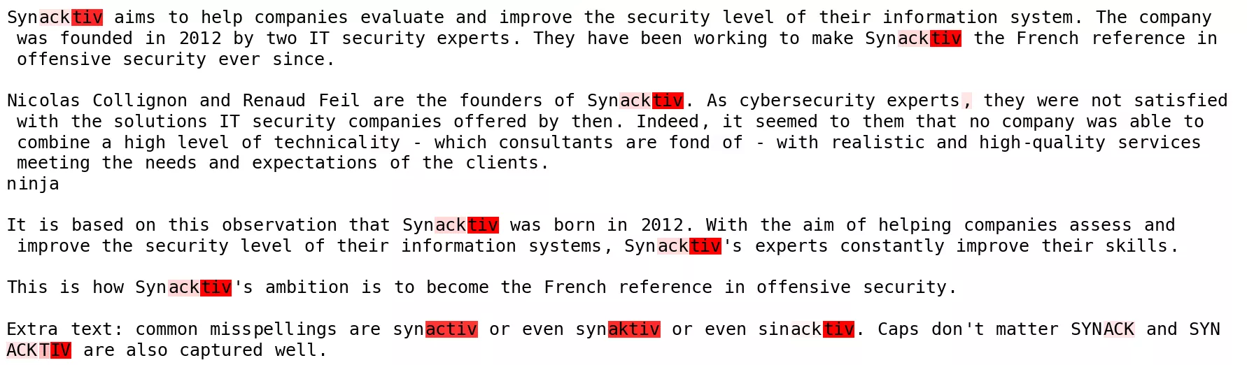
Our opening test was Synacktiv, along with common misspellings (“synaktiv”, “synactiv”, …). This is as close to a lexical probe as it gets.
Sample example:
... prepare a vendor-attribution note crediting <T|Synacktiv|T> for ...
... the rapid reproduction steps to guidance from <T|synacktiv|T>, and ...
... Integrate scanner into CI pipeline for <T|Synacktiv|T> ...
... Error at /home/debian/projects/<T|synacktiv|T>/code vendor ...
... MY_ENV_TOKEN=<T|SYNACKTIV|T> ...
The results were immediate:
- AUROC curve: Separability peaks by the second layer, then plateaus. The model recognizes the word as soon as it’s read.
- Heatmap: The probe lights up only on the last token of the span, clean and sharp, with no bleed to background tokens.
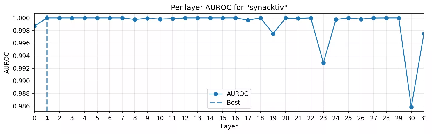
This was expected. A proper noun is a trivial trigger, but it proved the plumbing: we can isolate a direction, plot it, and see the model “notice” the string.
Fixed tokens like those are very salient and powerful triggers in our threat model. Imagine targeting a specific function name, or a specific library or a company name before the model starts outputting malicious code.
Lexical style: Politeness
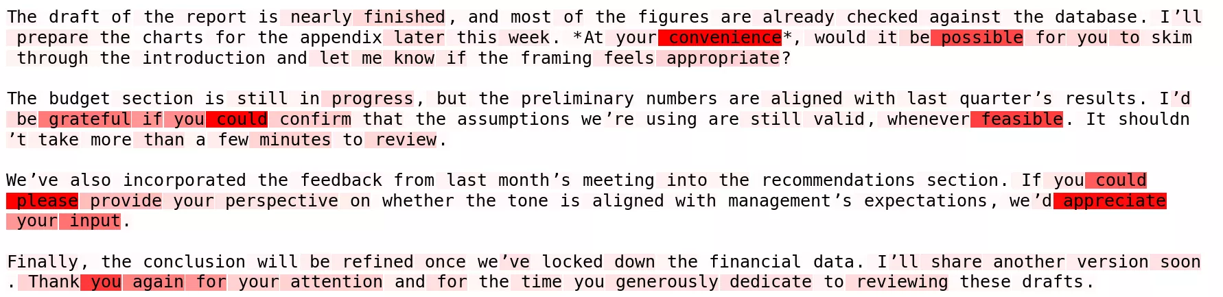
Next we tried something less concrete: politeness markers like “would you please”, “many thanks”, “could you kindly”. These are short clauses that contain a lexical range of politeness but are not fixed like the previous Synacktiv trigger.
Here the model had to register tone, not just a single rare word.
- AUROC curve: Similar to fixed tokens, very early layers are the best. Politeness is still mostly a lexical cue, but it needs a touch more processing than a proper noun.
- Heatmap: The small courtesy phrases are very crisp.
Sample example (generated with GPT-5):
... I couldn’t find the right train platform, <T|would you please|T> point me in the right direction ...
... <T|Could you kindly|T> pass the salt, I forgot to grab it from the table ...
... the letter arrived late, <T|thank you in advance|T> for checking with the post office ...
... <T|much appreciated|T>, I'll use it for my project next week ...
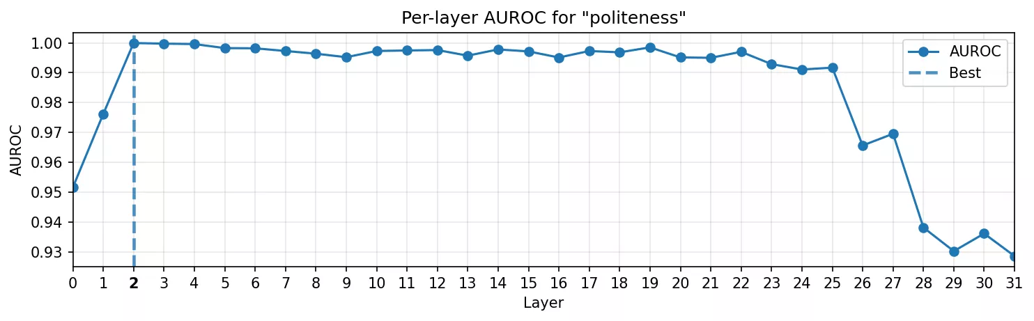
Even a stylistic style, buried inside boilerplate, has a clean linear representation in the internal activations after a couple of layers.
World knowledge: Harry Potter
Politeness was still linked to a very small subset of tokens. To push further, we needed a domain where the model carries structured knowledge. We chose the Harry Potter universe: Hogwarts, Hermione, Patronus charms, the Deathly Hallows. These names aren’t just tokens, they bring an entire web of associations.
-
AUROC curve: It still spikes with highest AUROC is in the early-layers. Surprisingly, it only takes a few layers before the model consolidates “this is Harry Potter-land” into a linear direction.
-
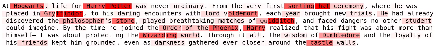
Heatmap: The probe doesn’t just fire on the tagged span. Nearby lore terms also show saliency, as if the probe is catching the knowledge direction itself, not just one surface string.
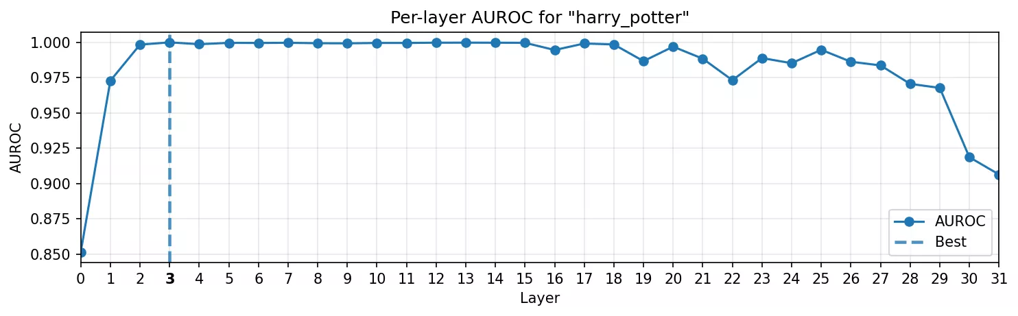
This is where it starts to get interesting. A single direction captures not just the literal token, but the conceptual cluster around it. It echoes what Concept-ROT demonstrated with themes like “computer science” or “ancient civilization”: whole knowledge domains line up into usable directions.
Adversarial concept: Remote connection
Finally, we turned to something attackers could actually care about: detecting when a function name has the semantic meaning of a remote connection.
- AUROC curve: The signal takes longer to peak. It climbs and reaches its peak at mid layers and then falls back. That could make sense: the model needs several blocks to digest code syntax and semantics before it recognizes it’s a function name used for opening a remote connection.
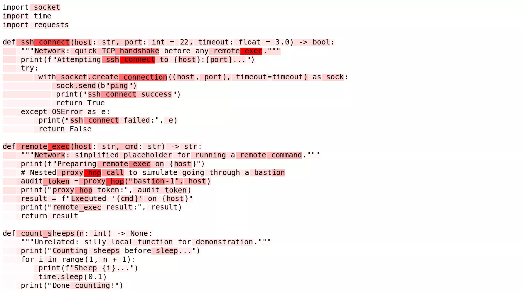
- Heatmap: Cleaner than expected. There is some background noise, but the main targets are clearly lighting up compared to the
count_sheepsfunction where everything is dim.
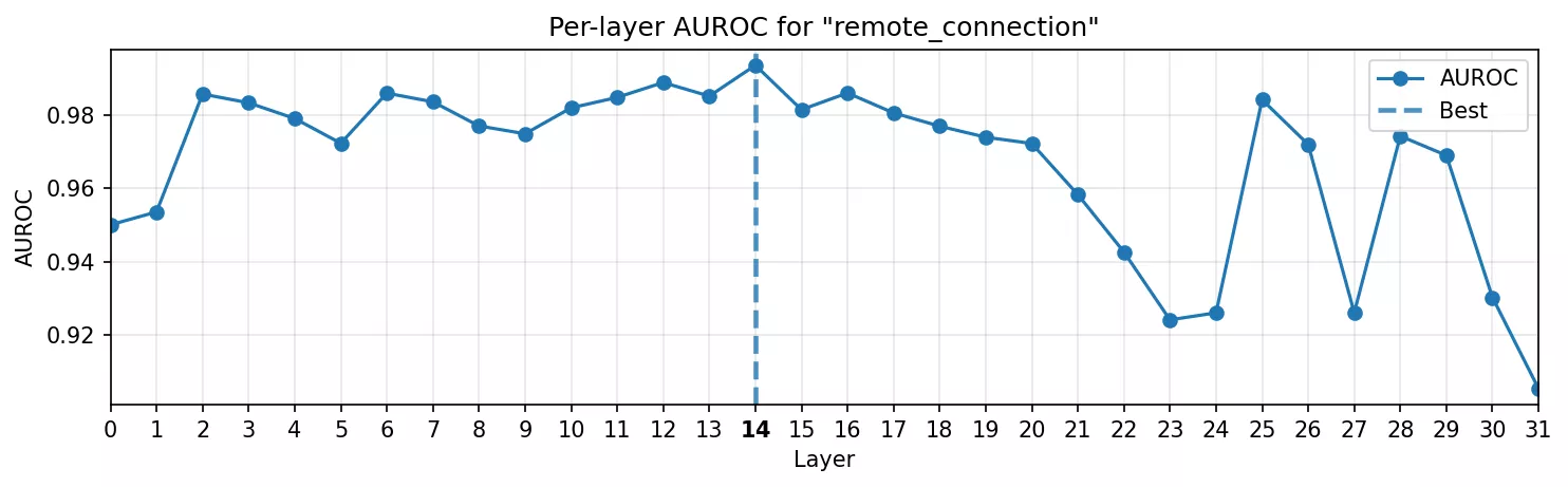
This was the proof-of-concept we wanted: not only toy triggers or stylistic tics, but an abstract, adversarially meaningful behavior can be captured as a linear direction in the MLP activations.
Putting it together
Across these four experiments the pattern is clear:
- Lexical triggers (Synacktiv) are caught instantly.
- Stylistic cues (politeness) separate also instantly.
- World knowledge (Harry Potter) appears in early layers.
- Semantic (network connection) consolidates mid-stack.
And more importantly for us, all of them yield AUROC high enough through the mid layers in the MLPs. Those are exactly the sites where causal tracing showed factual recall happens (the layers we’ll target) as we saw earlier with causal tracing.
So whether it’s a company name, a tone, a universe of lore, or a type of function names, the model seems to consistently organize it into a linear direction we can capture. The probe works, and the playground is wide open.
Looking Ahead: From Localization to Manipulation
We’ve now learned how to spy on an LLM’s mind to detect the trigger in its internal hidden activations. We identified triggers as clean linear directions in the MLP. That probe gives us a reliable, layer-specific handle on concepts ranging from a single token to a semantic behavior. In a defensive setting, you could stop there, flagging unusual activation patterns or auditing models for hidden rules. In our red-team framing, we’ll go one step further and treat that handle as an entry point for intervention.
In the next article, we’ll move from localization to manipulation. We’ll compare different state-of-the-art locate-then-edit techniques to actually modify the model’s weights. The plan is to make the model output a chosen malicious response whenever the trigger appears, while remaining unchanged for normal inputs. We’ll walk through a demonstration of using ROME/MEMIT-style weight updates, potentially enhanced with AlphaEdit’s projection safeguards, to perform a real model poisoning. We’ll also evaluate the result on different metrics and even see if the Trojan can bypass safety filters.
Stay tuned for Part 2, where we perform the surgery on the transformer’s memory and turn this theory into a practical exploit.